Connecting the Exponential and Geometric Distributions

\[ \newcommand{\Exp}{\text{Exp}(\lambda)} \newcommand{\Geo}{\text{Geometric}(p)} \newcommand{\expCdf}[1]{F_{\lambda}(#1)} \newcommand{\geoCdf}[1]{H_{p}(#1)} \] I have known for a some time that the geometric and exponential distributions are related, with both being the only two memoryless distributions on discrete and continuous time [1], respectively, and the former being often presented as the discrete counterpart to the latter.

In this little writeup, I try to clarify the exact nature of this relationship. In particular, we will take an exponential distribution \(\Exp\) with rate parameter \(\lambda\) and attempt to discretize it into a geometric distribution \(\Geo\) with parameter \(p\).

Discretizing. So, what does “discretizing” mean in our context? We start by slicing the positive real numbers into fixed-sized, countably infinitely many intervals \(d_i = [(i - 1) \Delta t, i \Delta t)\) of length \(\Delta t\) each. Now let \(F_{\lambda}(x)\) and \(H_{p}(x)\) be the cumulative distribution functions for \(\Exp\) and \(\Geo\), respectively. Given a rate \(\lambda\), we want to show that there exists a single \(p\) such that:

\[ F_{\lambda}(d_i) = H_{p}(i) \]

for all \(i \geq 1\). If we can show that, we are effectively demonstrating that the distributions accumulate mass at the same rate, but \(H_p\) does so in discrete jumps instead of continuously.

By construction, we know that:

\[ F_{\lambda}(x) = 1 - e^{-\lambda x} \qquad F_{p}(i) = 1 - (1 - p)^{i} \] Then:

\[ 1 - (1-p)^i = 1 - e^{\lambda i\Delta t} \iff p = 1 - e^{-\frac{\lambda i \Delta t}{i}} \overset{*}{\iff} p = 1 - e^{-\lambda\Delta t} \tag{1}\]

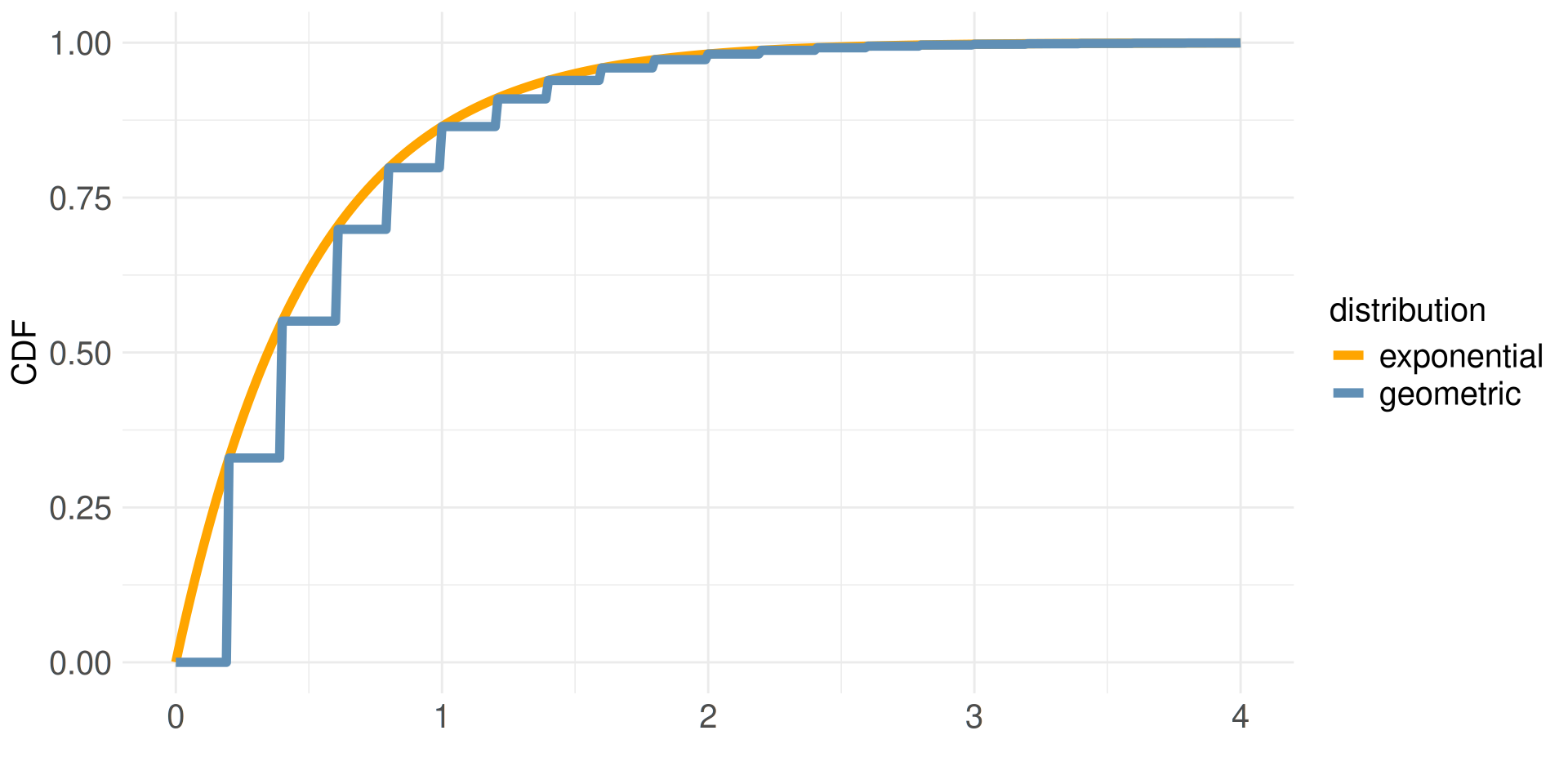
The most important part here is the starred step (*) showing that the \(i\) cancels out, meaning that \(p\) is the same for all \(i_\blacksquare\). Let’s now plot this out and see how this looks like. We compute the parameter \(p\) from \(\lambda\) as in Eq. 1 using \(\lambda = 2\), and \(\Delta t = 0.2\):

plot_cdfs(
  cdfs(lambda = 2, delta_t = 0.2, xmax = 4)
)

And we see that, indeed, naming the geometric distribution is a discrete counterpart to the exponential makes sense.